Ms excel Practical Question with solution; How to create score (mark) sheet of students.

Question:- Calculate following score sheet.

Symbol No	Eng	Nep	Mat	Sci	Percent	Grade

a. Use data validate to allow symbol number to have exactly 7 characters. (2)

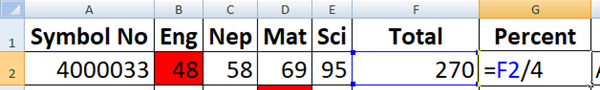
b. Apply conditional formatting to display marks in red color if it is smaller than 50. (2)

c. Calculate Percentage and Grade. Grade is awarded as below. (4)

    i. A+ if any of the marks obtained is more than 90.

   ii. A if percent is greater than 60.

  iii. B if percent is greater than 50.

  iv. C if percent is below 50 or any of the mark is below 60.

c. Apply Colorfull auto-format for the table. (2)

Solution:-

To display column in red color according to condition.

Step 1:- Select cell range B2:E6.

Step 2:- Go to Home Tab.

Step 3:- Click Conditional Fomatting under Styles Group.

Step 4:- Click Manage Rules. 

Step 5:- Click New Rule. 

Step 6:- Click Format only cells that contain. 

Step 7:- Select less than and value =50 

Step 8:- Click Format.

Step 9:- Select Background Color and Click OK button. 

Formulas for finding required information:-

Total (F2):-     =SUM(B2:E2) 

Percentage (G2):-   =F2/4 

Grade  (H2):-      =IF(G2>90,"A+",IF(G2>60,"A",IF(G2>50,"B",IF(OR(G2<50,G2<60),"C")))) 

To format table:-

Step 1:- Go to Home Tab.

Step 2:- Click Format as Table option under Styles Group. 

Step 3:- Choose any option that are required or fit yours problem. That’s all.